1 About the project
COMING SOON 🤓
2 Code
1
2
3
4
5
6
| # Source: https://www.geeksforgeeks.org/python-gender-identification-by-name-using-nltk/
# importing libraries
import random
from nltk.corpus import names
import nltk
import pandas as pd
|
Book Depository
This is where I have the nature history writers data here is the code for getting this data.
1
2
3
4
5
| # Import Bookdepository CSV
#authors = pd.read_csv("/Users/nat/Desktop/Code/Code Projects/Book-Gender/Data/Bookdepository/NaturalHistory-Bookdepository-2021.csv", dtype=str)
authors = pd.read_csv("/Users/nat/Desktop/Code/Code Projects/Book-Gender/Data/Bookdepository/NaturalHistory-Bookdepository-All.csv", dtype=str)
authors.head(5)
|
| Unnamed: 0 | authors | titles | date | year |
|---|
| 0 | 0 | Stephen Hawking | A Brief History Of Time | 20 Jan 2015 | 2015 |
|---|
| 1 | 1 | James Bowen | A Street Cat Named Bob | 23 Jan 2013 | 2013 |
|---|
| 2 | 2 | Peter Wohlleben | The Hidden Life of Trees | 22 Nov 2019 | 2019 |
|---|
| 3 | 3 | Raynor Winn | The Salt Path | 31 Jan 2019 | 2019 |
|---|
| 4 | 4 | Catherine D. Hughes | Little Kids First Big Book of Dinosaurs | 16 Aug 2018 | 2018 |
|---|
1
2
3
4
5
6
7
8
9
10
11
12
13
| # Create a colum for first names
authors["FirstName"] = ""
authors['FirstName'] = authors['authors'].str.split(" ")#1, expand=True
#authors['FirstName'][1][0] # 'Jeremy'
# Create an empty column for gender
authors["Gender"] = ""
# Drop unnecessary columns
authors.drop('Unnamed: 0', axis=1, inplace=True)
authors.head(5)
|
| authors | titles | date | year | FirstName | Gender |
|---|
| 0 | Stephen Hawking | A Brief History Of Time | 20 Jan 2015 | 2015 | [Stephen, Hawking] | |
|---|
| 1 | James Bowen | A Street Cat Named Bob | 23 Jan 2013 | 2013 | [James, Bowen] | |
|---|
| 2 | Peter Wohlleben | The Hidden Life of Trees | 22 Nov 2019 | 2019 | [Peter, Wohlleben] | |
|---|
| 3 | Raynor Winn | The Salt Path | 31 Jan 2019 | 2019 | [Raynor, Winn] | |
|---|
| 4 | Catherine D. Hughes | Little Kids First Big Book of Dinosaurs | 16 Aug 2018 | 2018 | [Catherine, D., Hughes] | |
|---|
NLTK Prediction
I used the name dataset from here
1
2
3
4
5
6
7
8
9
10
11
12
13
14
15
16
17
18
19
20
21
22
| def gender_features(word):
return {'last_letter':word[-1]}
# preparing a list of examples and corresponding class labels.
labeled_names = ([(name, 'Female') for name in names.words('/Users/nat/Desktop/Code/Code Projects/Book-Gender/Data/Names/Dataset2/Female.txt')]+
[(name, 'Male') for name in names.words('/Users/nat/Desktop/Code/Code Projects/Book-Gender/Data/Names/Dataset2/Male.txt')])
random.shuffle(labeled_names)
# we use the feature extractor to process the names data.
featuresets = [(gender_features(n), gender)
for (n, gender)in labeled_names]
# Divide the resulting list of feature
# sets into a training set and a test set.
train_set, test_set = featuresets[500:], featuresets[:500]
# The training set is used to
# train a new "naive Bayes" classifier.
classifier = nltk.NaiveBayesClassifier.train(train_set) # 76% accuracy
#print(nltk.classify.accuracy(classifier, train_set)) # Accuract is 0.7461467177257799
|
1
2
3
4
5
6
7
8
9
10
11
12
13
14
15
16
17
18
19
| for i in range(len(authors)): #iterate over rows
# Get the name
name = authors['FirstName'][i][0]
# If the authors' name is in our name dataset check gender
if name in open('/Users/nat/Desktop/Code/Code Projects/Book-Gender/Data/Names/Dataset2/AllNames.txt').read():
gender = classifier.classify(gender_features(name))
authors["Gender"][i] = str(gender)
# If the name is empty print unknown
elif name == 0:
authors["Gender"][i] = "Unknown"
# If the name is not in the database print unknown
else:
authors["Gender"][i] = "Unknown"
print('Done')
|
1
2
| # Check the table. Now it should have a designated/predicted gender for each author
authors.head(5)
|
| authors | titles | date | year | FirstName | Gender |
|---|
| 0 | Stephen Hawking | A Brief History Of Time | 20 Jan 2015 | 2015 | [Stephen, Hawking] | Male |
|---|
| 1 | James Bowen | A Street Cat Named Bob | 23 Jan 2013 | 2013 | [James, Bowen] | Male |
|---|
| 2 | Peter Wohlleben | The Hidden Life of Trees | 22 Nov 2019 | 2019 | [Peter, Wohlleben] | Male |
|---|
| 3 | Raynor Winn | The Salt Path | 31 Jan 2019 | 2019 | [Raynor, Winn] | Male |
|---|
| 4 | Catherine D. Hughes | Little Kids First Big Book of Dinosaurs | 16 Aug 2018 | 2018 | [Catherine, D., Hughes] | Female |
|---|
Save the Result
1
2
| authors.to_csv('/Users/nat/Desktop/Code/Code Projects/Book-Gender/Data/Bookdepository/NaturalHistory-All-Gender.csv')
|
Create Stat & Plot All The Data
1
2
| # You can observe the data with these commands
#authors.describe()
|
1
2
3
4
5
6
7
8
9
10
11
12
13
14
15
16
17
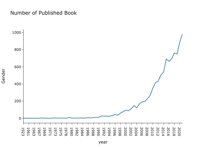
| import plotly.express as px
# Book number per year (the below will give a pandas series)
years_no= authors.groupby('year')['Gender'].count()
# Convert pandas series into a dataframe
df_years = pd.DataFrame(years_no)
df_years.reset_index(inplace=True)
# Drop the books that had publishing dates in the future.
df_years = df_years[df_years["year"].str.contains("2024")==False]
df_years = df_years[df_years["year"].str.contains("2023")==False]
df_years = df_years[df_years["year"].str.contains("2022")==False] # I will also remove 2022 as we are in the beginnign of this year
# Plot the data
fig = px.line(df_years, x=df_years['year'], y=df_years['Gender'], title='Number of Published Book')
fig.show()
|
![Graph1]()
Gender Gap in the all (retrieved) nature book published
1
2
3
4
5
6
7
8
9
10
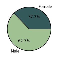
| f = authors['Gender'].value_counts()['Female'] # All: 3465
m = authors['Gender'].value_counts()['Male'] # All: 5836
u = authors['Gender'].value_counts()['Unknown'] # All: 659
stat = pd.DataFrame({
'Female': [f],
'Male': [m]
#'Unknown': [u]
})
stat
|
1
2
3
4
5
6
7
8
9
10
11
12
13
14
15
16
17
18
19
20
21
22
23
24
25
26
27
28
29
| from matplotlib import pyplot as plt
mylabels = ["Female", "Male"]
mycolors = ["#34595a", "#a0c293"]
#controls default text size
plt.rc('font', size=15)
# plot size
#plt.rcParams["figure.figsize"] = [10, 15]
#set title font to size 50
plt.rc('axes', titlesize=50)
plt.pie(stat,
labels = mylabels,
autopct ='%1.1f%%',
colors = mycolors,
wedgeprops = {"edgecolor" : "black",
'linewidth': 2,
'antialiased': True})
#plt.legend(loc='upper left')
#plt.title('Gender Gap')
# Save figure
#plt.savefig('/Users/nat/Desktop/gender-gap-All.png', dpi = 100)
# Display the graph onto the screen
plt.show()
|
![Graph2]()
Gender Gap Yearly Analysis
1
2
3
4
5
6
7
8
| # Filter data
df_2020 = authors[(authors['year'] == '2020')]
df_2015 = authors[(authors['year'] == '2015')]
df_2010 = authors[(authors['year'] == '2010')]
df_2005 = authors[(authors['year'] == '2005')]
df_2000 = authors[(authors['year'] == '2000')]
df_1995 = authors[(authors['year'] == '1995')]
df_1990 = authors[(authors['year'] == '1990')]
|
1
2
3
4
5
6
7
8
9
10
11
12
13
14
15
16
17
18
19
20
21
22
23
| f2 = df_2020['Gender'].value_counts()['Female']
m2 = df_2020['Gender'].value_counts()['Male']
u2 = df_2020['Gender'].value_counts()['Unknown']
f7 = df_2015['Gender'].value_counts()['Female']
m7 = df_2015['Gender'].value_counts()['Male']
u7 = df_2015['Gender'].value_counts()['Unknown']
f8 = df_2010['Gender'].value_counts()['Female']
m8 = df_2010['Gender'].value_counts()['Male']
u8 = df_2010['Gender'].value_counts()['Unknown']
f9 = df_2005['Gender'].value_counts()['Female']
m9 = df_2005['Gender'].value_counts()['Male']
u9 = df_2005['Gender'].value_counts()['Unknown']
f10 = df_2000['Gender'].value_counts()['Female']
m10 = df_2000['Gender'].value_counts()['Male']
u10 = df_2000['Gender'].value_counts()['Unknown']
f11 = df_1995['Gender'].value_counts()['Female']
m11 = df_1995['Gender'].value_counts()['Male']
u11 = df_1995['Gender'].value_counts()['Unknown']
|
1
2
3
4
5
6
7
8
| # Create your dataframes
every_5 = pd.DataFrame({
'Year': [2020, 2015, 2010, 2005, 2000, 1995],
'Female': [f2, f7, f8, f9, f10, f11],
'Male': [m2, m7, m8, m9, m10, m11]
#'Unknown': [u]
})
every_5
|
| Year | Female | Male |
|---|
| 0 | 2020 | 358 | 465 |
|---|
| 1 | 2015 | 263 | 383 |
|---|
| 2 | 2010 | 107 | 225 |
|---|
| 3 | 2005 | 58 | 99 |
|---|
| 4 | 2000 | 31 | 59 |
|---|
| 5 | 1995 | 12 | 19 |
|---|
1
2
3
4
5
6
7
8
9
10
11
12
13
14
15
16
17
18
19
20
21
22
23
24
25
26
27
28
29
30
31
32
33
34
35
36
37
38
39
| import plotly.graph_objects as go
# labels={'trace 0': "hello", 'trace 1': "hi"}
# set up plotly figure
fig = go.Figure()
# add line / trace 1 to figure
fig.add_trace(go.Scatter(
x=every_5['Year'],
y=every_5['Female'],
hovertext=every_5['Female'],
hoverinfo="text",
marker=dict(
color="black"
),
showlegend=True,
line_width=3
))
# add line / trace 2 to figure
fig.add_trace(go.Scatter(
x=every_5['Year'],
y=every_5['Male'],
hovertext=every_5['Male'],
hoverinfo="text",
marker=dict(
color="green"
),
showlegend=True,
line_width=3
))
# Source: https://www.geeksforgeeks.org/plotly-how-to-show-legend-in-single-trace-scatterplot-with-plotly-express/
fig['data'][0]['showlegend'] = True
fig['data'][0]['name'] = 'Female'
fig['data'][1]['name'] = 'Male'
fig.show(renderer="png")
|
![Graph3]()
1
2
3
4
5
6
7
8
9
10
11
12
13
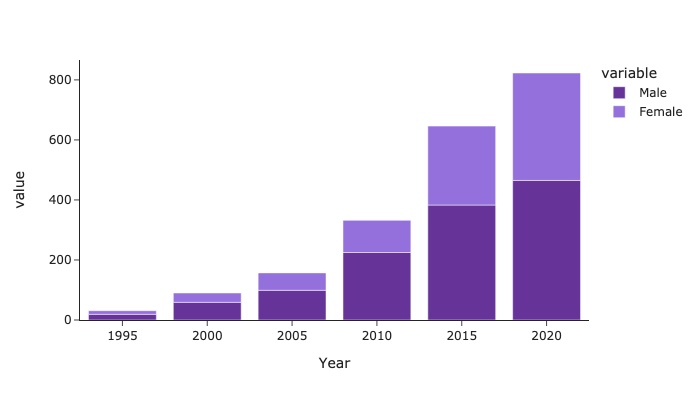
| import plotly.express as px
import pandas as pd
import plotly.graph_objs as go
fig = px.bar(every_5,
x=every_5['Year'],
y=[every_5['Male'], every_5['Female']],
height=400, width=700,
color_discrete_map= {"Male": "RebeccaPurple",
"Female": "MediumPurple"},
template="simple_white"
)
fig.show(renderer="png")
|
![Graph4]()